3D 张量并行

作者: Zhengda Bian, Yongbin Li

前置教程

示例代码

ColossalAI-Examples - 3D Tensor Parallelism

相关论文

Maximizing Parallelism in Distributed Training for Huge Neural Networks

引言

3D 张量并行是一种将神经网络模型的计算并行化，以期望获得最佳通信成本优化的方法。

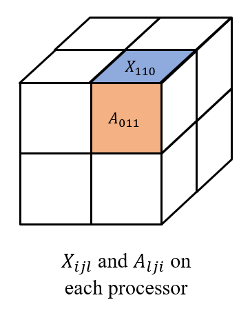
我们还是以线性层 $Y = XA$ 为例。给定 $P=q \times q \times q$ 个处理器（必要条件）, 如 $q=2$ , 我们把输入 $X$ 和权重 $A$ 划分为

\left[\begin{matrix} X_{000} & X_{001} \\ X_{010} & X_{011} \\ X_{100} & X_{101} \\ X_{110} & X_{111} \end{matrix} \right] \text{~and~} \left[\begin{matrix} A_{000} & A_{001} & A_{010} & A_{011} \\ A_{100} & A_{101} & A_{110} & A_{111} \end{matrix} \right] \text{~respectively,}

其中每个 $X_{ijl}$ 和 $A_{lji}$ 都被存储在处理器 $(i,j,l)$ 上, 如下图所示。

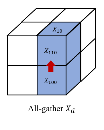
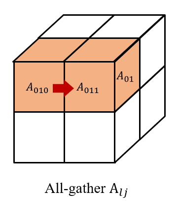
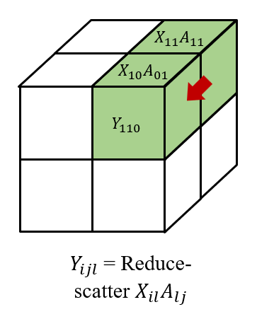
然后我们在 $(i, 0...q,l)$ 上收集 $X_{ijl}$ , 以及在 $(0...q, j, l)$ 上收集 $A_{lji}$ 。因此，我们在每个处理器 $(i,j,l)$ 上都有 $X_{il}$ 和 $A_{lj}$ 以获得 $X_{il}A_{lj}$ 。最后，我们在 $(i, j, 0...q)$ 对结果进行 reduce-scatter 得到 $Y_{ijl}$ , 形成

Y= \left[\begin{matrix} Y_{000} & Y_{001} \\ Y_{010} & Y_{011} \\ Y_{100} & Y_{101} \\ Y_{110} & Y_{111} \end{matrix} \right].

我们还需要注意，在后向传播中, 我们需要 all-gather 梯度 $\dot{Y_{ijl}}$ , 然后 reduce-scatter 梯度 $\dot{X_{il}}=\dot{Y_{ij}}A_{lj}^T$ and $\dot{A_{lj}}=X_{il}^T\dot{Y_{ij}}$ 。

效率

给定 $P=q \times q \times q$ 个处理器, 我们展现理论上的计算和内存成本，以及基于环形算法的3D张量并行的前向和后向的通信成本。

计算	内存 (参数)	内存 (activations)	通信 (带宽)	通信 (时延)
$O(1/q^3)$	$O(1/q^3)$	$O(1/q^3)$	$O(6(q-1)/q^3)$	$O(6(q-1))$

使用

为了使我们的模型能够实现3D张量并行，例如在8个 GPU 上，我们需要配置如下的并行设置。

CONFIG = dict(parallel=dict(
    data=1,
    pipeline=1,
    tensor=dict(size=8, mode='3d'),
))

然后 Colossal-AI 会自动对所有来自 colossalai.nn 的层应用3D张量并行。

让我们定义一个由两层多层感知器 (MLP) 组成的模型，如下所示。

import colossalai
import colossalai.nn as col_nn
import torch
from colossalai.utils import print_rank_0

class MLP(torch.nn.Module):
    def __init__(self, dim: int = 256):
        super().__init__()
        intermediate_dim = dim * 4
        self.dense_1 = col_nn.Linear(dim, intermediate_dim)
        print_rank_0(f'Weight of the first linear layer: {self.dense_1.weight.shape}')
        self.activation = torch.nn.GELU()
        self.dense_2 = col_nn.Linear(intermediate_dim, dim)
        print_rank_0(f'Weight of the second linear layer: {self.dense_2.weight.shape}')
        self.dropout = col_nn.Dropout(0.1)

    def forward(self, x):
        x = self.dense_1(x)
        print_rank_0(f'Output of the first linear layer: {x.shape}')
        x = self.activation(x)
        x = self.dense_2(x)
        print_rank_0(f'Output of the second linear layer: {x.shape}')
        x = self.dropout(x)
        return x

在8个 GPU 上启动 Colossal-AI 并建立模型。

parser = colossalai.get_default_parser()
colossalai.launch(config=CONFIG,
                  rank=args.rank,
                  world_size=args.world_size,
                  local_rank=args.local_rank,
                  host=args.host,
                  port=args.port)

m = MLP()

我们将会看到 MLP 模型中被划分的参数（如权重）的形状。

Weight of the first linear layer: torch.Size([128, 256])
Weight of the second linear layer: torch.Size([512, 64])

第一个线性层的完整权重形状应该为 [256, 1024]. 经过3D并行划分后，它在每个 GPU 上变成了 [128, 256] 。同样地，第二层将权重 [1024, 256] 划分为 [512, 64].

我们可以用一些随机输入来运行这个模型。

from colossalai.context import ParallelMode
from colossalai.core import global_context as gpc
from colossalai.utils import get_current_device

x = torch.randn((16, 256), device=get_current_device())
# partition input
torch.distributed.broadcast(x, src=0)
x = torch.chunk(x, 2, dim=0)[gpc.get_local_rank(ParallelMode.PARALLEL_3D_WEIGHT)]
x = torch.chunk(x, 2, dim=0)[gpc.get_local_rank(ParallelMode.PARALLEL_3D_INPUT)]
x = torch.chunk(x, 2, dim=-1)[gpc.get_local_rank(ParallelMode.PARALLEL_3D_OUTPUT)]
print_rank_0(f'Input: {x.shape}')

x = m(x)

然后我们可以看到 activation 结果的形状。

Input: torch.Size([4, 128])
Output of the first linear layer: torch.Size([4, 512])
Output of the second linear layer: torch.Size([4, 128])

3D并行中的 activation 张量都是同时在 $q^2$ 行和 $q$ 列分割的。例如，第一个线性层的输出是 [4, 512], 而第二层的输出为 [4, 128]。注意，虽然这里3D并行的结果与2.5D并行的结果形状相同，但每个划分的内容是不同的。

3D 张量并行

引言​

效率​

使用​

引言

效率

使用