Paradigms of Parallelism
Author: Shenggui Li, Siqi Mai
Introduction
With the development of deep learning, there is an increasing demand for parallel training. This is because that model and datasets are getting larger and larger and training time becomes a nightmare if we stick to single-GPU training. In this section, we will provide a brief overview of existing methods to parallelize training. If you wish to add on to this post, you may create a discussion in the GitHub forum.
Data Parallel
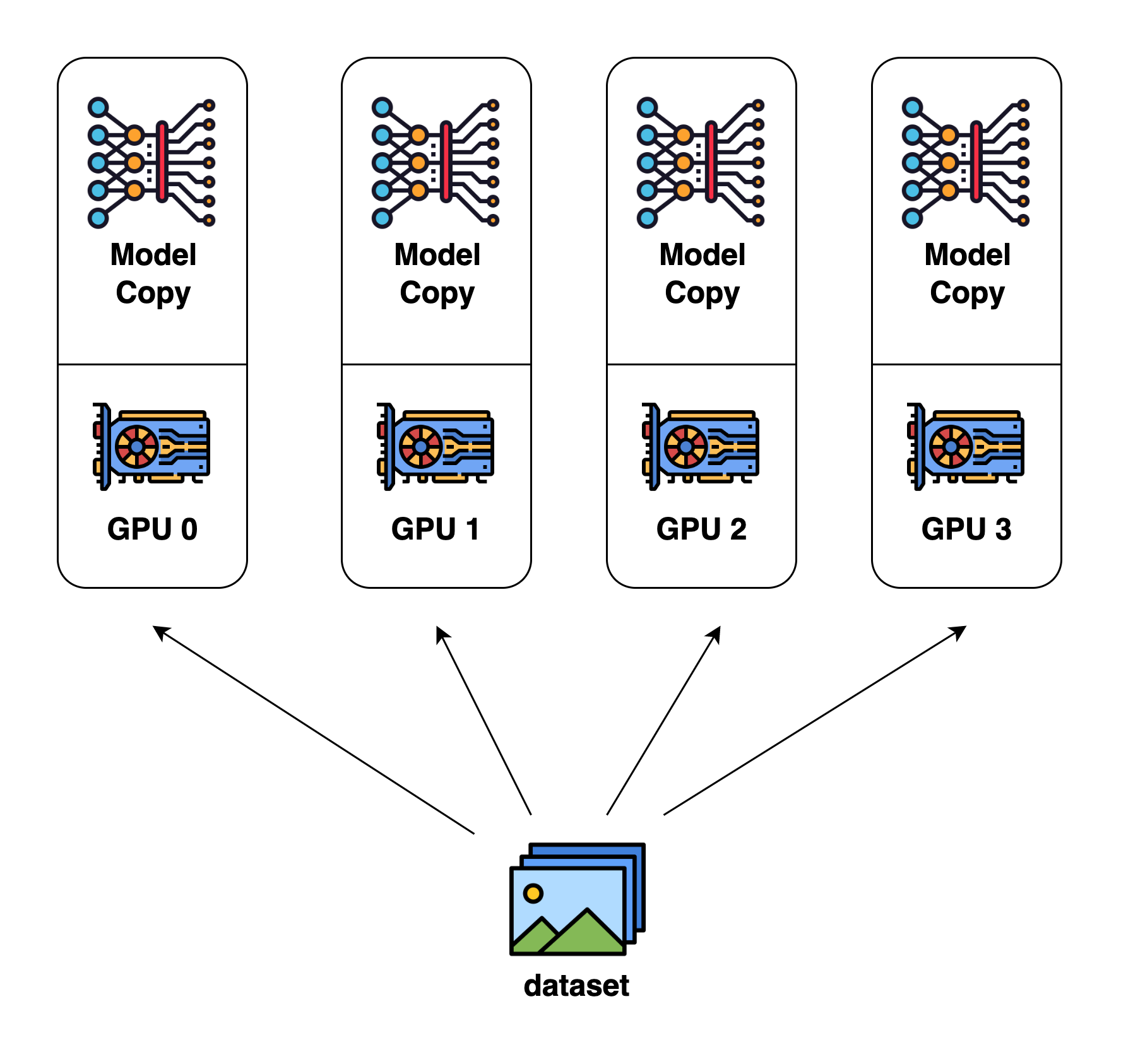
Data parallel is the most common form of parallelism due to its simplicity. In data parallel training, the dataset is split into several shards, each shard is allocated to a device. This is equivalent to parallelize the training process along the batch dimension. Each device will hold a full copy of the model replica and trains on the dataset shard allocated. After back-propagation, the gradients of the model will be all-reduced so that the model parameters on different devices can stay synchronized.
Model Parallel
In data parallel training, one prominent feature is that each GPU holds a copy of the whole model weights. This brings redundancy issue. Another paradigm of parallelism is model parallelism, where model is split and distributed over an array of devices. There are generally two types of parallelism: tensor parallelism and pipeline parallelism. Tensor parallelism is to parallelize computation within an operation such as matrix-matrix multiplication. Pipeline parallelism is to parallelize computation between layers. Thus, from another point of view, tensor parallelism can be seen as intra-layer parallelism and pipeline parallelism can be seen as inter-layer parallelism.
Tensor Parallel
Tensor parallel training is to split a tensor into N chunks along a specific dimension and each device only holds 1/N
of the whole tensor while not affecting the correctness of the computation graph. This requires additional communication
to make sure that the result is correct.
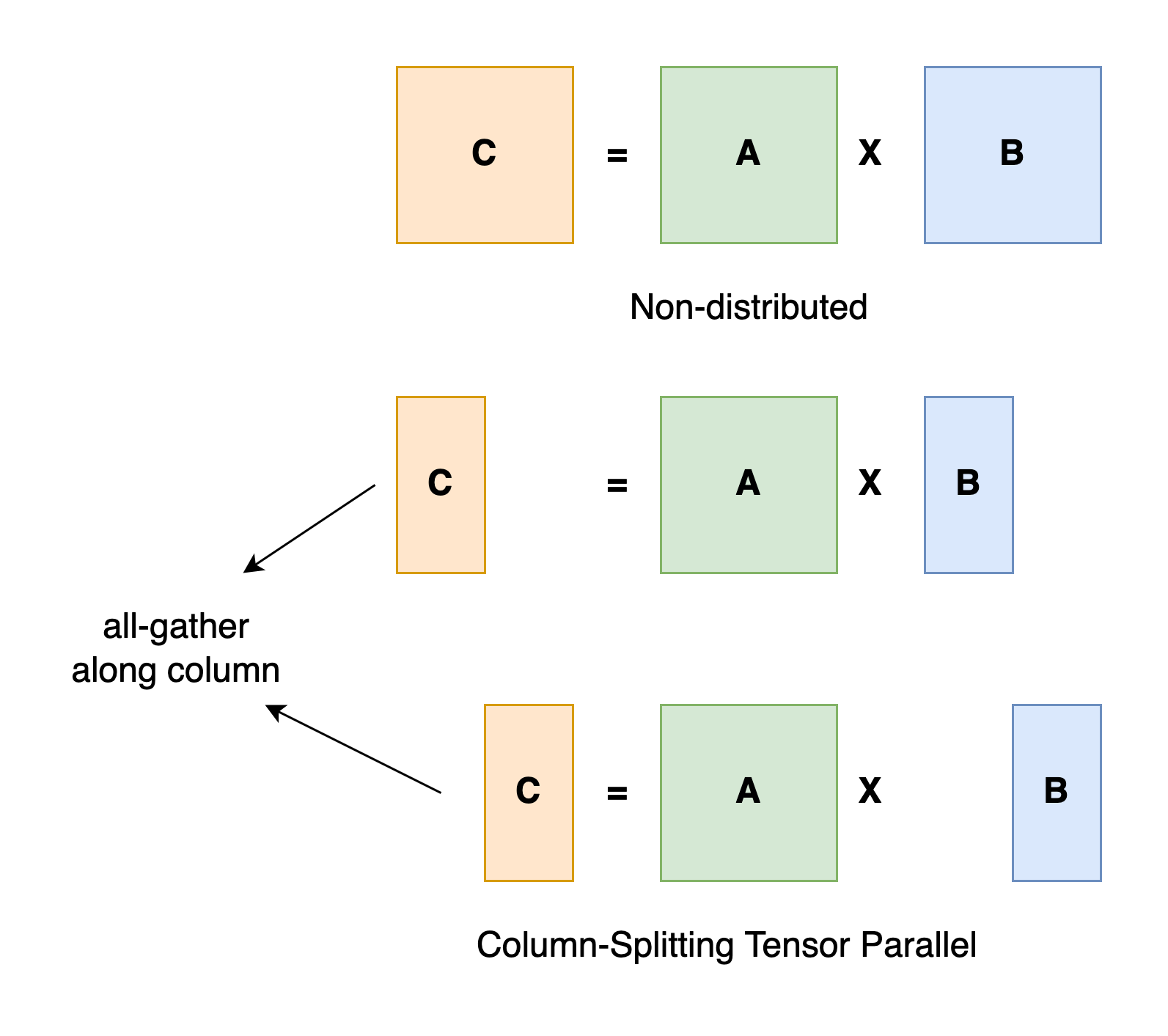
Taking a general matrix multiplication as an example, let's say we have C = AB. We can split B along the column dimension
into [B0 B1 B2 ... Bn] and each device holds a column. We then multiply A with each column in B on each device, we
will get [AB0 AB1 AB2 ... ABn]. At this moment, each device still holds partial results, e.g. device rank 0 holds AB0.
To make sure the result is correct, we need to all-gather the partial result and concatenate the tensor along the column
dimension. In this way, we are able to distribute the tensor over devices while making sure the computation flow remains
correct.
In Colossal-AI, we provide an array of tensor parallelism methods, namely 1D, 2D, 2.5D and 3D tensor parallelism. We will
talk about them in detail in advanced tutorials.
Related paper:
- GShard: Scaling Giant Models with Conditional Computation and Automatic Sharding
- Megatron-LM: Training Multi-Billion Parameter Language Models Using Model Parallelism
- An Efficient 2D Method for Training Super-Large Deep Learning Models
- 2.5-dimensional distributed model training
- Maximizing Parallelism in Distributed Training for Huge Neural Networks
Pipeline Parallel
Pipeline parallelism is generally easy to understand. If you recall your computer architecture course, this indeed exists in the CPU design.
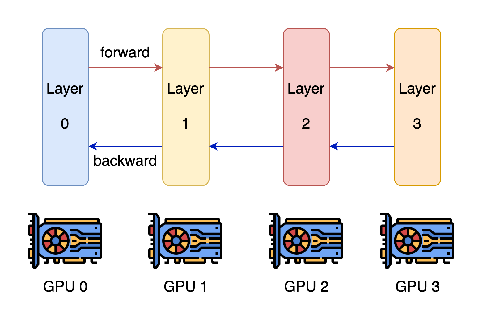
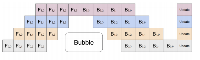
The core idea of pipeline parallelism is that the model is split by layer into several chunks, each chunk is given to a device. During the forward pass, each device passes the intermediate activation to the next stage. During the backward pass, each device passes the gradient of the input tensor back to the previous pipeline stage. This allows devices to compute simultaneously, and increases the training throughput. One drawback of pipeline parallel training is that there will be some bubble time where some devices are engaged in computation, leading to waste of computational resources.
Related paper:
- PipeDream: Fast and Efficient Pipeline Parallel DNN Training
- GPipe: Efficient Training of Giant Neural Networks using Pipeline Parallelism
- Megatron-LM: Training Multi-Billion Parameter Language Models Using Model Parallelism
- Chimera: Efficiently Training Large-Scale Neural Networks with Bidirectional Pipelines
Sequence Parallelism
Sequence parallelism is a parallel strategy that partitions along the sequence dimension, making it an effective method for training long text sequences. Mature sequence parallelism methods include Megatron’s sequence parallelism, DeepSpeed-Ulysses sequence parallelism, and ring-attention sequence parallelism.
Megatron SP:
This sequence parallelism method is implemented on top of tensor parallelism. On each GPU in model parallelism, the samples are independent and replicated. For parts that cannot utilize tensor parallelism, such as non-linear operations like LayerNorm, the sample data can be split into multiple parts along the sequence dimension, with each GPU computing a portion of the data. Then, tensor parallelism is used for the linear parts like attention and MLP, where activations need to be aggregated. This approach further reduces activation memory usage when the model is partitioned. It is important to note that this sequence parallelism method can only be used in conjunction with tensor parallelism.
DeepSpeed-Ulysses:
In this sequence parallelism, samples are split along the sequence dimension and the all-to-all communication operation is used, allowing each GPU to receive the full sequence but only compute the non-overlapping subset of attention heads, thereby achieving sequence parallelism. This parallel method supports fully general attention, allowing both dense and sparse attention. all-to-all is a full exchange operation, similar to a distributed transpose operation. Before attention computation, samples are split along the sequence dimension, so each device only has a sequence length of N/P. However, after using all-to-all, the shape of the qkv subparts becomes [N, d/p], ensuring the overall sequence is considered during attention computation.
Ring Attention:
Ring attention is conceptually similar to flash attention. Each GPU computes only a local attention, and finally, the attention blocks are reduced to calculate the total attention. In Ring Attention, the input sequence is split into multiple chunks along the sequence dimension, with each chunk handled by a different GPU or processor. Ring Attention employs a strategy called "ring communication," where kv sub-blocks are passed between GPUs through p2p communication for iterative computation, enabling multi-GPU training on ultra-long texts. In this strategy, each processor exchanges information only with its predecessor and successor, forming a ring network. This allows intermediate results to be efficiently transmitted between processors without global synchronization, reducing communication overhead.
Related paper: Reducing Activation Recomputation in Large Transformer Models DeepSpeed Ulysses: System Optimizations for Enabling Training of Extreme Long Sequence Transformer Models Ring Attention with Blockwise Transformers for Near-Infinite Context
Optimizer-Level Parallel
Another paradigm works at the optimizer level, and the current most famous method of this paradigm is ZeRO which stands for zero redundancy optimizer. ZeRO works at three levels to remove memory redundancy (fp16 training is required for ZeRO):
- Level 1: The optimizer states are partitioned across the processes
- Level 2: The reduced 32-bit gradients for updating the model weights are also partitioned such that each process only stores the gradients corresponding to its partition of the optimizer states.
- Level 3: The 16-bit model parameters are partitioned across the processes
Related paper:
Parallelism on Heterogeneous System
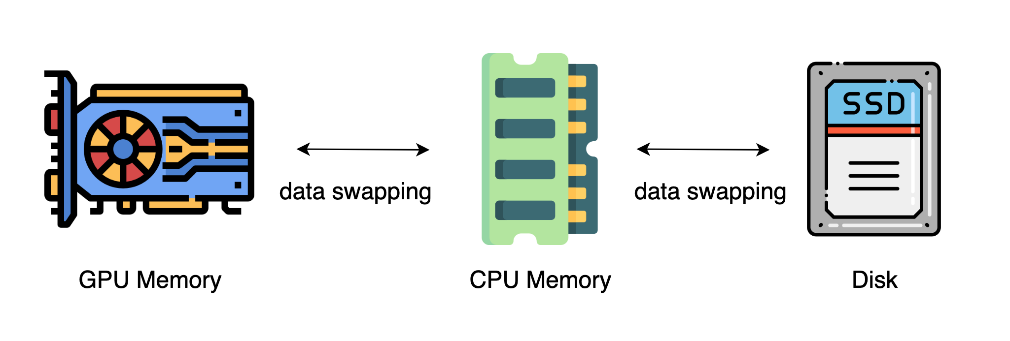
The methods mentioned above generally require a large number of GPU to train a large model. However, it is often neglected that CPU has a much larger memory compared to GPU. On a typical server, CPU can easily have several hundred GB RAM while each GPU typically only has 16 or 32 GB RAM. This prompts the community to think why CPU memory is not utilized for distributed training.
Recent advances rely on CPU and even NVMe disk to train large models. The main idea is to offload tensors back to CPU memory or NVMe disk when they are not used. By using the heterogeneous system architecture, it is possible to accommodate a huge model on a single machine.
Related paper: